Gradient Descent on Loss Landscapes

Visualizing how optimizer trajectories behave on non-convex loss surfaces — saddle points, local minima, and escape dynamics.

Setup

%matplotlib inline
import numpy as np
import matplotlib.pyplot as plt
from matplotlib.colors import LinearSegmentedColormap

plt.rcParams.update({
    'figure.facecolor': '#111118',
    'axes.facecolor': '#1a1a24',
    'axes.edgecolor': '#1a1a24',
    'axes.labelcolor': '#8888aa',
    'xtick.color': '#8888aa',
    'ytick.color': '#8888aa',
    'text.color': '#e8e8f0',
    'font.family': 'monospace',
})

print('Ready.')

Ready.

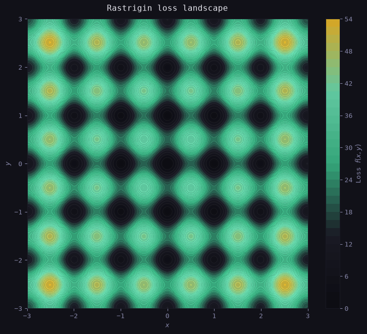
A Non-Convex Test Landscape

We use a 2D version of the Rastrigin function as our loss surface: f(x, y) = 20 + x^2 + y^2 - 10(\cos 2\pi x + \cos 2\pi y)

def rastrigin(x, y):
    return 20 + x**2 + y**2 - 10*(np.cos(2*np.pi*x) + np.cos(2*np.pi*y))

x = np.linspace(-3, 3, 400)
y = np.linspace(-3, 3, 400)
X, Y = np.meshgrid(x, y)
Z = rastrigin(X, Y)

# Custom colormap: ink → mint
cmap = LinearSegmentedColormap.from_list(
    'site', ['#0a0a0f', '#1a1a24', '#3abf8a', '#6ee7b7', '#fbbf24']
)

fig, ax = plt.subplots(figsize=(8, 7))
cf = ax.contourf(X, Y, Z, levels=40, cmap=cmap, alpha=0.85)
ax.contour(X, Y, Z, levels=20, colors='white', alpha=0.08, linewidths=0.5)

plt.colorbar(cf, ax=ax, label='Loss $f(x,y)$')
ax.set_title('Rastrigin loss landscape', color='#e8e8f0', pad=12)
ax.set_xlabel('$x$'); ax.set_ylabel('$y$')

plt.tight_layout()
plt.show()
print('Loss landscape rendered.')

Loss landscape rendered.