Variational Quantum Circuits

An introduction to parameterized quantum circuits, the parameter-shift rule, and barren plateaus — with working code examples.

Overview

A variational quantum circuit (VQC) is a parameterized quantum circuit U(\boldsymbol{\theta}) = \prod_{l=1}^{L} U_l(\theta_l) where each U_l is a unitary gate that depends on a classical parameter \theta_l \in \mathbb{R}.

The goal is to minimize a cost function \mathcal{L}(\boldsymbol{\theta}) = \langle 0 | U^\dagger(\boldsymbol{\theta})\, H\, U(\boldsymbol{\theta}) | 0 \rangle where H is a Hermitian observable.

%matplotlib inline
import numpy as np
import matplotlib.pyplot as plt

# Apply a dark style that matches the site
plt.rcParams.update({
    'figure.facecolor': '#111118',
    'axes.facecolor': '#1a1a24',
    'axes.edgecolor': '#1a1a24',
    'axes.labelcolor': '#8888aa',
    'xtick.color': '#8888aa',
    'ytick.color': '#8888aa',
    'grid.color': '#1a1a24',
    'text.color': '#e8e8f0',
    'font.family': 'monospace',
})

print('Libraries loaded.')

Libraries loaded.

The Parameter-Shift Rule

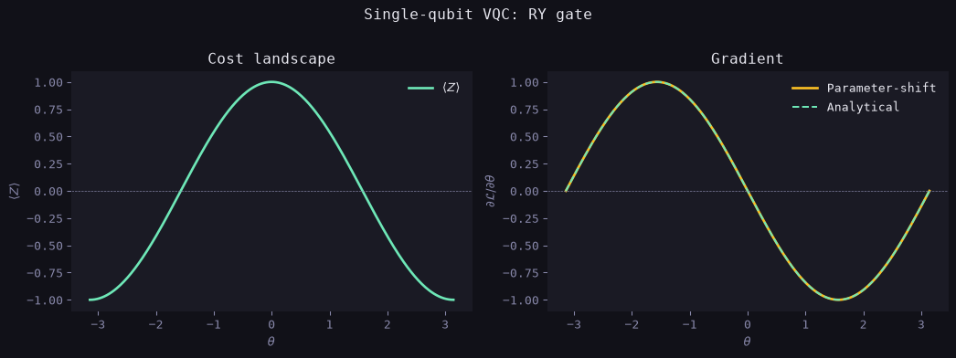
For gates of the form U(\theta) = e^{-i\theta G/2} where G^2 = I, the gradient can be computed exactly via two circuit evaluations:

\frac{\partial \mathcal{L}}{\partial \theta_k} = \frac{1}{2}\left[\mathcal{L}\!\left(\theta_k + \frac{\pi}{2}\right) - \mathcal{L}\!\left(\theta_k - \frac{\pi}{2}\right)\right]

Below we simulate this for a simple 1-qubit expectation value.

# Simulate <Z> = cos(theta) for a single RY gate applied to |0>
def expectation(theta):
    """<Z> after RY(theta)|0>"""
    return np.cos(theta)

def parameter_shift_grad(theta):
    """Exact gradient via parameter-shift rule."""
    return 0.5 * (expectation(theta + np.pi/2) - expectation(theta - np.pi/2))

thetas = np.linspace(-np.pi, np.pi, 300)
cost   = expectation(thetas)
grad   = parameter_shift_grad(thetas)
true_g = -np.sin(thetas)  # analytical derivative

fig, (ax1, ax2) = plt.subplots(1, 2, figsize=(11, 4))

# Left: cost landscape
ax1.plot(thetas, cost, color='#6ee7b7', linewidth=2, label=r'$\langle Z \rangle$')
ax1.axhline(0, color='#8888aa', linewidth=0.5, linestyle='--')
ax1.set_xlabel(r'$\theta$')
ax1.set_ylabel(r'$\langle Z \rangle$')
ax1.set_title('Cost landscape', color='#e8e8f0')
ax1.legend(framealpha=0)
ax1.set_facecolor('#1a1a24')

# Right: gradient
ax2.plot(thetas, grad,   color='#fbbf24', linewidth=2,   label='Parameter-shift')
ax2.plot(thetas, true_g, color='#6ee7b7', linewidth=1.5, linestyle='--', label='Analytical')
ax2.axhline(0, color='#8888aa', linewidth=0.5, linestyle='--')
ax2.set_xlabel(r'$\theta$')
ax2.set_ylabel(r"$\partial\mathcal{L}/\partial\theta$")
ax2.set_title('Gradient', color='#e8e8f0')
ax2.legend(framealpha=0)
ax2.set_facecolor('#1a1a24')

fig.suptitle('Single-qubit VQC: RY gate', color='#e8e8f0', fontsize=12, y=1.01)
plt.tight_layout()
plt.show()

Barren Plateaus

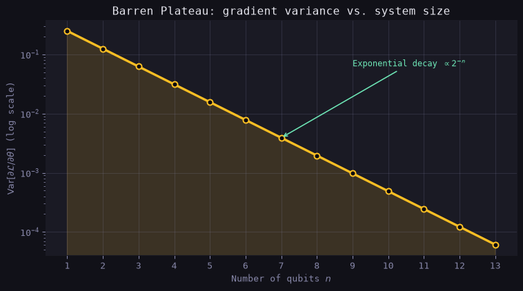
A central challenge in training VQCs is the barren plateau phenomenon: for deep random circuits on n qubits, the variance of the gradient vanishes exponentially, \text{Var}\!\left[\frac{\partial \mathcal{L}}{\partial \theta_k}\right] \in O(2^{-n}).

The plot below illustrates how gradient variance decays with circuit depth.

np.random.seed(42)

n_qubits_list = np.arange(1, 14)
# Gradient variance decays as ~2^(-n) for global cost functions
variance = 2.0 ** (-n_qubits_list.astype(float)) * 0.5

fig, ax = plt.subplots(figsize=(8, 4.5))

ax.semilogy(n_qubits_list, variance,
            color='#fbbf24', linewidth=2.5, marker='o',
            markersize=6, markerfacecolor='#0a0a0f',
            markeredgecolor='#fbbf24', markeredgewidth=1.5)

ax.fill_between(n_qubits_list, variance, alpha=0.15, color='#fbbf24')

ax.set_xlabel('Number of qubits $n$')
ax.set_ylabel(r'$\text{Var}[\partial\mathcal{L}/\partial\theta]$ (log scale)')
ax.set_title('Barren Plateau: gradient variance vs. system size', color='#e8e8f0')
ax.set_xticks(n_qubits_list)
ax.grid(True, alpha=0.2, color='#8888aa')
ax.set_facecolor('#1a1a24')

# Annotation
ax.annotate('Exponential decay $\\propto 2^{-n}$',
            xy=(7, variance[6]), xytext=(9, variance[2]),
            arrowprops=dict(arrowstyle='->', color='#6ee7b7', lw=1.2),
            color='#6ee7b7', fontsize=9)

plt.tight_layout()
plt.show()

Summary

Concept	Key result
Parameter-shift gradient	Exact, hardware-compatible
Barren plateaus	Variance \propto 2^{-n} for global cost
Mitigation strategies	Local cost functions, structured ansätze, QNGO

Next: Noise-resilient gradient estimation — how shot noise and hardware errors compound with barren plateaus.